
Manufacturing inventory management usually fails in a quiet place: the on-hand balance says a component exists, but the bin is empty. Production releases the job, purchasing sees no shortage, and the line discovers the truth only after setup. The shortage is visible. The bad transaction that caused it may be weeks old.
The cure is not a larger spreadsheet or a new vendor demo. It is an operating policy for what gets counted, when replenishment starts, how much uncertainty to buffer, and who closes each discrepancy. Software can enforce that policy later. It cannot invent one for you.
Direct answer — What is manufacturing inventory management?
Manufacturing inventory management is the practice of controlling raw materials, work in progress, finished goods, and maintenance supplies so production can meet demand without tying up avoidable cash. It combines accurate records, item classification, replenishment triggers, safety stock, cycle counting, and ownership rules. MRP or ERP can calculate and record the plan, but neither fixes unreliable counts, weak receiving, or uncontrolled material movement.
Key Takeaways
- Inventory accuracy is the gate. Reorder formulas only work when physical stock and records agree.
- Raw material, WIP, finished goods, and MRO spares need different controls because each fails differently.
- Reorder point answers when to buy; safety stock covers uncertainty; EOQ estimates an economical order size.
- ABC analysis should set attention and count frequency, but production criticality must override dollar value.
- Move to software after locations, units, transaction ownership, and counting discipline are stable.
| Method | What it controls | When it fits | When it fails |
|---|---|---|---|
| Min/max | Lower and upper stock limits | Stable, inexpensive repeat items | Limits are not reviewed after demand or lead time changes |
| Reorder point | When replenishment starts | Repeat demand with measurable lead time | Open orders, allocations, or variable lead time are ignored |
| Safety stock | Demand and supply uncertainty | Items where a stockout carries real cost | A guessed buffer hides poor supplier or forecast performance |
| EOQ | Economic replenishment quantity | Steady demand and known order and holding costs | Job-shop demand, price breaks, or lead times move sharply |
| ABC analysis | Control effort by annual usage value | Large item masters that need priorities | A cheap but line-stopping part is treated as unimportant |
| Cycle counting | Record accuracy and process errors | Continuous control without a plant-wide shutdown | Teams adjust balances but never investigate root causes |
What Manufacturing Inventory Management Controls
Manufacturing inventory management is the discipline of keeping the right material, in the right state and location, available when production or shipment needs it. The job spans four control loops: plan requirements, receive and identify stock, record every movement, and reconcile the record to physical reality.
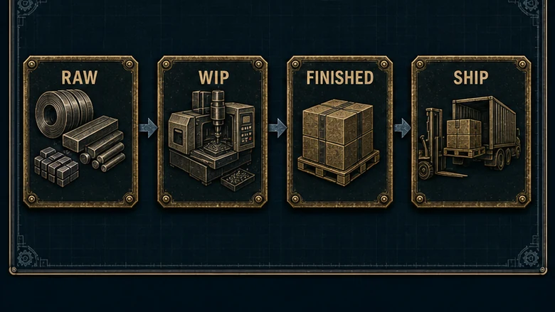
Targets should not be set SKU by SKU in isolation. The supply review inside sales and operations planning turns the demand plan, capacity constraints, supplier risk, and working-capital limits into inventory targets that operations can defend. A reorder point is then a local execution rule for that broader decision, not the strategy itself.
Raw material is a supplier and timing problem
Raw material includes purchased components, ingredients, packaging, and subassemblies waiting to enter production. Control begins with item identity, unit of measure, approved location, lot or serial needs, lead time, minimum order quantity, and the transaction that records receipt. One incorrect case-to-each conversion can create a larger planning error than a weak forecast.
Supplier reliability belongs in the policy. A low-cost part with one approved source and a twelve-week lead time deserves more attention than its purchase price suggests. The supplier qualification and continuity decisions belong in strategic sourcing; the inventory rule translates those decisions into a buffer, review cadence, or second-source trigger.
WIP is a flow and location problem
Work in progress is material that has been issued or transformed but is not yet finished. WIP becomes invisible when operators move a tote without reporting the move, combine jobs, backflush against a wrong bill of materials, or leave completed operations open. The result is not merely an accounting error. Scheduling sees capacity and material in the wrong state.
Control WIP at defined handoff points rather than at every foot of travel. Record issue to the job, completion of the operation, quantity good, quantity scrapped, and the next controlled location. If the transaction burden is so high that operators skip it, the design is too granular for the floor.
Finished goods are a demand and promise problem
Finished goods are completed units ready for sale or shipment. Make-to-stock plants control them through forecast, service level, shelf life, and allocation rules. Make-to-order shops may hold little finished stock, but they still need clear status for inspection hold, available, allocated, staged, and shipped. Calling all five states “on hand” creates false availability.
MRO spares are a criticality problem
Maintenance, repair, and operating supplies should be separated from production material even when they share a storeroom. A bearing, drive, fuse, lubricant, or filter is consumed by asset risk, not customer demand. Classify MRO by the consequence of a stockout, repair lead time, interchangeability, and whether the part can be repaired, not only by annual spend.
Make Inventory Accuracy the First Control
Inventory accuracy is the percentage of counted item-location records whose physical quantity agrees with the system within a stated tolerance. It is a process metric, not a warehouse vanity score, because every material plan, available-to-promise date, shortage message, and financial value inherits the accuracy of the underlying record.
The scale of the decision is visible in the U.S. Census Bureau’s July 2, 2026 manufacturing report: manufacturers held $962.0 billion of inventory in May, up 0.2% for an eighth consecutive monthly increase, with an inventories-to-shipments ratio of 1.47. Your plant is smaller, but the same question holds: how much of the number is usable stock rather than a ledger assumption?
Inventory record accuracy = Correct count lines ÷ Total count lines × 100Define “correct” before reporting the percentage. Exact-match counting is appropriate for serialized, regulated, or high-value items. A stated unit tolerance may be defensible for bulk fasteners or liquids, but a hidden tolerance makes the metric easy to improve without improving control.
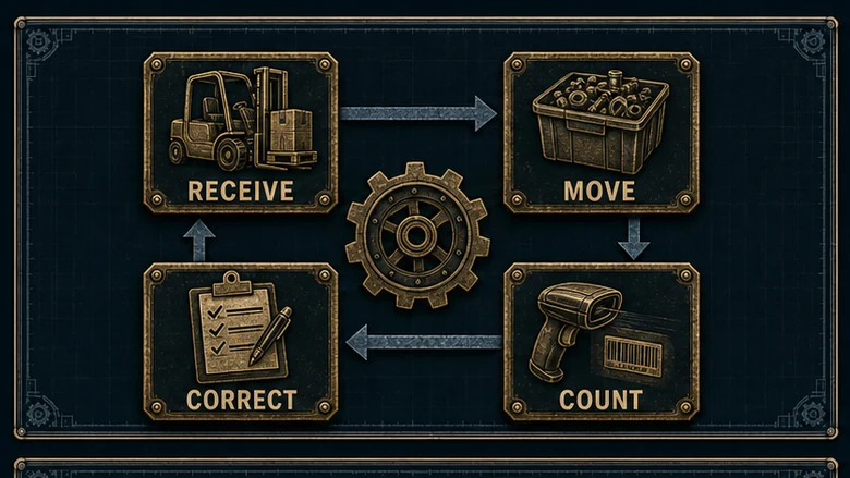
Set the record before tuning formulas
Start with four master-data decisions: one stocking unit, one base unit of measure, named locations, and a status vocabulary that people can see on the floor. Then define who records receipts, transfers, issues, returns, scrap, completions, and shipments. Shared responsibility usually means no responsibility.
A useful benchmark is procedural rather than aspirational. The U.S. GAO guide to inventory count practices describes a leading company that required facilities to sustain accuracy above 95% and demonstrate sound receiving, manufacturing, movement, and shipping controls before replacing annual wall-to-wall counts with cycle counting. The number was a gate attached to process evidence.
IMPORTANT
If physical inventory is only 82% accurate, the missing 18% is not a software problem. Freeze the affected zone, reconcile it, and trace the transaction failure before changing reorder parameters.
Measure the error, then name its cause
Do not stop at “adjusted +12.” Record whether the variance came from receiving, unit conversion, unlabeled location, unreported issue, scrap, return, production completion, shipment, or theft and damage. A cycle count program that only posts adjustments is a recurring cleanup service for an unchanged process.
Track accuracy by item class and location, adjustment value, repeat-error rate, and time to close the cause. Plant-wide accuracy can hide a bad receiving cage or a family of components whose units are routinely confused.
Choose a Replenishment Method by Demand Pattern
A replenishment method is the rule that decides when supply should be created and how much should be ordered or produced. The best rule is the simplest one that represents demand, lead time, order constraints, and stockout consequence without creating more maintenance than the item deserves.
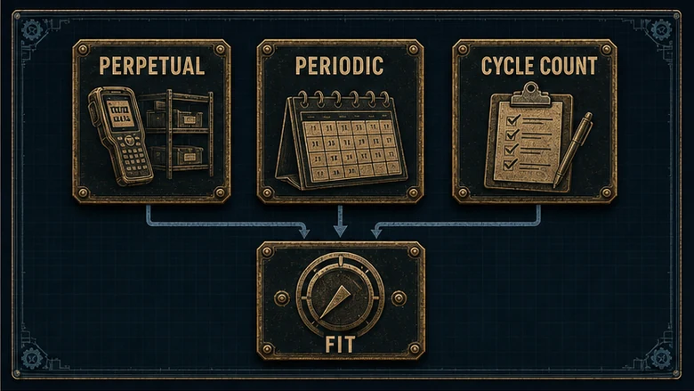
Use min/max for stable repeat items
Set a minimum that triggers review or replenishment and a maximum that caps the post-receipt position. This works for predictable consumables, packaging, and common hardware. It fails when the limits sit untouched after volume, lead time, lot size, or scrap changes. Every limit needs an owner and a review date.
For standardized consumables with a capable supplier, vendor-managed inventory can move the bin check and replenishment decision to the supplier. That reduces buyer touches, but it still needs agreed minimums, maximums, ownership, consumption visibility, and an exception path. VMI does not remove the policy; it changes who executes it.
Use reorder point for repeat demand with lead time
A reorder point triggers supply when the inventory position reaches expected demand during replenishment lead time plus a buffer. Use inventory position, not merely shelf quantity: on hand plus firm inbound supply minus allocations and backorders. Otherwise an open purchase order or committed job can make the trigger lie.
The purchase order is only half of replenishment. Approval, receipt, inspection, three-way match, and invoice control sit in the procure-to-pay process. If receipts wait two shifts to be posted, the system will keep proposing stock that is already on the dock.
Use EOQ as a cost estimate, not a command
Economic order quantity estimates the order size that minimizes annual ordering and holding cost. The Virginia Tech inventory model shows both the formula and its assumptions: demand and lead time are constant, replenishment is effectively immediate, and unit cost does not change with quantity.
EOQ = √((2 × Annual demand × Cost per order) ÷ Annual holding cost per unit)Suppose annual demand is 12,000 units, each order costs $60 to place and receive, and annual holding cost is $3 per unit. EOQ is about 693 units. Treat that as a cost-centered starting point. Round for pack size, minimum order quantity, shelf life, space, cash, and production reality.
EOQ often breaks in a high-mix job shop because demand is intermittent, purchased material is job-specific, and one order may combine several projects. Lot-for-lot buying against released demand can be safer there. The right answer is allowed to be less mathematically elegant.
Use JIT only where replenishment is dependable
Just-in-time is a synchronized pull system, not a slogan for cutting every buffer. Toyota describes JIT as making only what is needed, when needed, in the amount needed, while maintaining the minimum stock required for the replenishment loop. The Toyota Production System explanation also makes the dependency clear: linked processes and suppliers must move in cadence.
Use JIT for repeat flow with stable quality, short and visible lead time, disciplined signals, and recovery options. Keep a deliberate buffer where lead time is long, supply is concentrated, demand is lumpy, or a stockout stops an expensive line. Inventory is waste when it hides a weak process. It is insurance when the risk is named and priced.
PRO TIP
Use min/max for simple consumables, reorder point for repeat items with measurable lead time, lot-for-lot for job-specific demand, and JIT only where the replenishment loop has proved reliable.
Calculate Reorder Point and Safety Stock
To calculate a reorder point, estimate average demand during replenishment lead time and add safety stock for the variation you choose to protect. Use the same time unit for demand and lead time, and calculate by item-location because both demand and supplier performance can differ by plant.
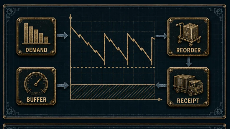
Reorder point = Average daily demand × Average lead time in days + Safety stockFor stable lead time and reasonably continuous demand, a basic statistical buffer uses the service factor, daily-demand standard deviation, and square root of lead time.
Safety stock = z × Daily demand standard deviation × √(Lead time)The Oracle inventory-optimization documentation uses a 1.65 z-score for a 95% service level and warns that normal-distribution results become approximate for intermittent, promotional, seasonal, or skewed demand. That warning matters more than the decimal precision.
Work a simple example
A component averages 40 units per day, supplier lead time averages eight days, and daily demand standard deviation is six units. At a 95% cycle-service target, safety stock is 1.65 × 6 × √8, or about 28 units. Reorder point is then 40 × 8 + 28, or 348 units.
The trigger does not mean “buy 348.” It means create or release supply when inventory position reaches 348. The order quantity comes from lot-for-lot demand, a fixed quantity, EOQ, pack size, minimum order quantity, or another approved rule.
Model lead-time variation when it is material
If supplier lead time moves, a demand-only buffer understates exposure. Use demand and lead-time history together, or adopt a conservative maximum-usage method until enough clean history exists. Do not bury supplier lateness inside a permanent buffer. Measure it, escalate it, and review whether sourcing or transport needs to change.
Recalculate after a sustained demand shift, supplier change, engineering revision, pack-size change, service-policy change, or a repeated stockout. A parameter without a review trigger becomes another stale field.
Use ABC Analysis Without Ignoring Criticality
ABC analysis ranks items by annual usage value so control effort follows financial exposure. Calculate annual usage value for each item, sort from highest to lowest, and classify the cumulative value into A, B, and C bands. The bands are management choices, not universal laws.
Annual usage value = Annual demand × Unit cost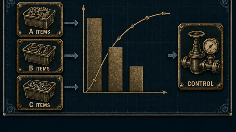
Work the classification from value
| Item | Annual demand | Unit cost | Annual usage value | Share | Initial class |
|---|---|---|---|---|---|
| Servo drive | 40 | $900 | $36,000 | 45% | A |
| Aluminum casting | 800 | $25 | $20,000 | 25% | A |
| Shipping carton | 20,000 | $0.80 | $16,000 | 20% | B |
| Bearing kit | 400 | $20 | $8,000 | 10% | C |
The four-item example totals $80,000. The servo drive and casting create 70% of annual usage value, so they receive A-level review. The carton receives B attention, and the bearing kit begins in C. In a real item master, choose cutoffs after looking at the curve rather than forcing every plant into 80/15/5.
Overlay criticality before setting control
Value alone can misclassify a cheap seal, fuse, fastener, or sensor that stops the only bottleneck machine. Add a criticality flag for safety, regulatory, line-stop, single-source, long-lead, and no-substitute exposure. Promote the control level when operational consequence is higher than the dollar class suggests.
Use the combined class to set count frequency, approval threshold, supplier review, location security, and parameter review. A items may be counted weekly or monthly; B items monthly or quarterly; C items less often. The schedule should respond to observed error, not tradition.
Replace the Annual Count With Cycle Counting
Cycle counting is a continuous control that reconciles selected item-location records throughout the year, investigates variances, and corrects the process that produced them. It can reduce disruption compared with a single wall-to-wall count, but only after receiving, movement, and transaction controls are stable enough to support it.
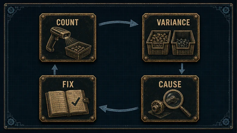
Run your first controlled cycle count
How to run a first cycle count
Count one bounded location, reconcile it without showing the expected quantity to the counter, and close the transaction cause before resuming normal movement.
Select one bounded location
Choose a rack, cage, or bin family that can be isolated and completed in one session. Avoid an entire warehouse for the first run.
Freeze material movement
Pause receipts, issues, transfers, and picks for the location, or timestamp every transaction so the count has a clear cutoff.
Issue a blind count sheet
Give the counter the item and location without the expected quantity. Record unit of measure, lot, serial, status, and observed quantity.
Recount material differences
Use a second person for differences above the approved tolerance or value threshold. Confirm neighboring bins and unit conversions before adjustment.
Trace the transaction cause
Check recent receipts, issues, transfers, scrap, completions, and shipments. Assign one cause code and one owner to each confirmed variance.
Post and close corrective action
Approve the quantity adjustment, correct the label or workflow, release the location, and schedule a verification count for repeated errors.
Count to learn, not merely to reconcile
Schedule more counts where value, criticality, transaction volume, or error history is high. Random selection is useful for testing whether apparently clean areas stay clean. Event-triggered counts after a negative balance, emergency issue, major variance, or location move catch failures close to the event that caused them.
Receiving errors should feed the same correction loop as invoice and purchase-order exceptions. When inspection hold, accepted quantity, and system receipt differ, the inventory team and purchasing team need one owner for the handoff, not two competing balances.
Control MRO Spares and Know When Software Helps
MRO inventory control protects asset availability with the smallest defensible investment in spares. The right policy combines asset criticality, failure mode, installed population, repairability, supplier lead time, shelf life, and substitute availability. Consumption history alone misses the rare part whose absence causes the worst outage.
Set a spares policy by consequence
Hold an on-site spare when failure stops a constrained or safety-critical asset, replenishment exceeds tolerated downtime, and no tested substitute or repair path exists. Pool or buy on demand when the part is common, interchangeable, quickly supplied, or attached to redundant equipment. Mark repaired, serviceable, failed, and quarantined spares as different statuses.
Do not let MRO become a museum. Review no-movement stock, superseded part numbers, cannibalized assemblies, shelf-life items, and spares for retired assets. Obsolete stock is not protection; it is evidence that the policy did not follow the asset base.
Move beyond a spreadsheet at the right trigger
A spreadsheet can work when the item list is small, one person owns every transaction, there is one location, and counts are frequent. It starts failing when several people move stock, units or lots matter, jobs reserve components, multiple locations share material, or purchase and production orders must update availability.
At that point, define requirements before opening a vendor list. The existing manufacturing inventory software buyer guide owns the system comparison, named vendors, and pricing. This page owns the operating practice. Keeping those intents separate prevents a software shortlist from replacing the policy it should enforce.
Connect the policy to MRP or ERP
MRP translates demand, bills of material, inventory, lead time, and order policies into planned supply. ERP adds purchasing, finance, sales, and shared transactions around it. The MRP versus ERP boundary matters when choosing system scope, but both depend on the same inputs: trustworthy balances, controlled locations, current lead times, and approved replenishment parameters.
The practical order is accuracy, policy, ownership, then automation. Reverse it and the new system produces faster shortage messages, faster excess orders, and more convincing reports built on the same weak record.
Frequently Asked Questions
Inventory management in manufacturing controls materials from receipt through production and shipment. It sets identification, location, movement, counting, replenishment, and exception rules for raw material, work in progress, finished goods, and MRO supplies. Its purpose is reliable production and delivery with a defensible amount of cash tied up in stock.
Raw material has not entered production, WIP has been issued or transformed but is not complete, and finished goods have passed production and are ready for sale or shipment. The distinction matters because each stage has different ownership, valuation, location, status, and replenishment signals. One generic “on hand” balance hides those differences.
Safety stock is a deliberate buffer held above expected demand during replenishment lead time. It protects a chosen service level against demand or supply variation. It should be calculated from clean history and reviewed when demand, lead time, sourcing, or stockout consequence changes. A guessed buffer can hide the process that needs correction.
Multiply average demand per day by average replenishment lead time in days, then add safety stock. Apply the trigger to inventory position: on hand plus firm inbound supply minus allocations and backorders. Use consistent units and calculate by item-location. Revisit the result after a sustained demand, supplier, pack-size, or service-policy change.
ABC analysis ranks items by annual usage value, calculated as annual demand multiplied by unit cost, so the highest financial exposure receives the most control. Manufacturers should overlay operational criticality before setting count frequency or buffers. A low-cost fuse that stops the bottleneck machine may need A-level control despite its C-level spend.
